The CISL Consulting Services Group ran numerous Weather Research and Forecasting (WRF) modeling system jobs on the Cheyenne supercomputer. The jobs included large and small runs with different domain sizes and time steps.
The scaling analysis provided in the next section may be helpful in answering questions such as:
Is it possible to solve a problem with such-and-such resolution in a timely manner?
I will have the results more quickly if I use more cores, but with this resolution will my run be in the efficient strong-scaling regime, an intermediate one, or in the very inefficient one dominated by I/O and initialization instead of computing?
Numbers from the figures below can help you develop some back-of-the-envelope estimates of what will happen if you increase or decrease the core counts of your runs. From there, you can find a core count that is optimal in terms of time-to-solution and in terms of your allocation.
While these plots provide some guidance, you do need to run some tests on Cheyenne or a comparable system if you're preparing an allocation request. Test runs can help support the validity of your core-hour estimate for your own physics parameterization. They can also help you account for the overhead from initialization and I/O. (Different I/O settings and frequency will affect your runs differently.)
Moreover, if you are concerned primarily with performance, use the latest Intel compiler and the SGI MPT library that is available on Cheyenne. This combination gave us the best performance as observed during our experiments when running WRF with various compilers and MPI libraries. The simulations below use WRFV4.0 compiled with Intel 18.0.1 and SGI's MPT 2.18.
Page contents
Also see these links for related documentation and additional information on preparing allocation requests:
Scaling results
Figure 1 shows scaling results from four different simulations: Hurricane Maria at 1km and 3km resolutions and the official CONUS benchmarks from (link no longer available) at 12km and 2.5km resolution. The CONUS benchmark uses the CONUS physics suite introduced from WRFv3.9 instead of the older physics combination used in the official benchmark. Note that both axes are logarithmic, so a small distance between points corresponds to a large difference in values.
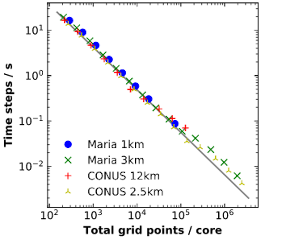
Figure 1
Notice the range of the x-axis. Total grid points per core varies from ~100 to ~10^6. This means that as grid points per core is reduced, the number of nodes increases, and vice-versa. When expressing the scaling as a function of WRF grid points per core, all the cases scaled similarly on Cheyenne.
WRF has linear strong scaling. This means the computational part of WRF is making effective use of the parallel computational resources available to it. Increasing the number of cores a run uses decreases the computation time proportionately – while initialization and I/O time may increase – and about the same number of core-hours are used for computation.
On the side of the plot where there are no blue or red points, the limiting factor is available memory. An increasingly large part of the domain must be held in the physical memory of each node, causing a lower core-count limit when the memory needed exceeds available memory.
Run-time results
Figure 2 below shows the total run time for WRF jobs with increasing numbers of cores. A core count of 36,864 corresponds to 1,024 nodes on Cheyenne. The results are based on simulations of Hurricane Maria at 1km resolution having a single output file, which used a domain of about 372 million grid points.
The total run time of WRF can be broken down into the initialization time, computation time, and output writing time. As illustrated, initialization and writing output times remain relatively fixed, increasing only slightly as you move to larger core counts. The numbers below may vary depending on the number of restart and output files your simulations have, but we expect the trend to be similar.
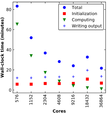
Figure 2