The Cheyenne environment supports the use of NCAR Command Language (NCL) both interactively and in batch mode to analyze and visualize data.
As described below, to use NCL in the Cheyenne environment you will log in to Cheyenne or Casper, then:
- Start an interactive job on Casper and execute the NCL script from that window, or
- Submit a batch job to execute an NCL script.
Follow the instructions below to get started, and customize the scripts and commands as necessary to work with your own data.
Other resources
See the NCL web site for complete documentation of the language's extensive analysis and visualization capabilities.
See the NCL Applications page for links to hundreds of complete NCL scripts that you can download and modify as needed.
Page contents
Interactive use
To start an interactive window from which to modify and execute NCL scripts, log in to Cheyenne.
ssh -X username@cheyenne.ucar.edu
Start a job on Casper as described in this documentation.
When your job starts, load the default module for NCL.
module load ncl
Modify your NCL script if necessary using a UNIX editor, and execute it as shown here, substituting the name of your own NCL script for script_name.ncl.
ncl script_name.ncl
Submitting a batch script
If you expect running your NCL script to take longer than you would want to work interactively — overnight, for example — submit your NCL script in a batch job so it can run unattended. See Starting jobs on Casper nodes for batch job script examples and other details.
When your batch script is ready, use the qsub command and the name of your script file.
qsub script_name
You might also find command files useful for performing a number of related NCL tasks in parallel. See this documentation for information about command files.
Visualization examples
Example 1
Make an NCL script file named contour_ts_line.ncl using the sample script below.
When you run it on Casper, it will create a simple line contour plot (Figure 1) using a sample CMIP5 NetCDF data file in the /glade/u/sampledata/ncl/CESM/CAM5 directory. The output to your working directory will be a graphic file called contour_ts_line.png.
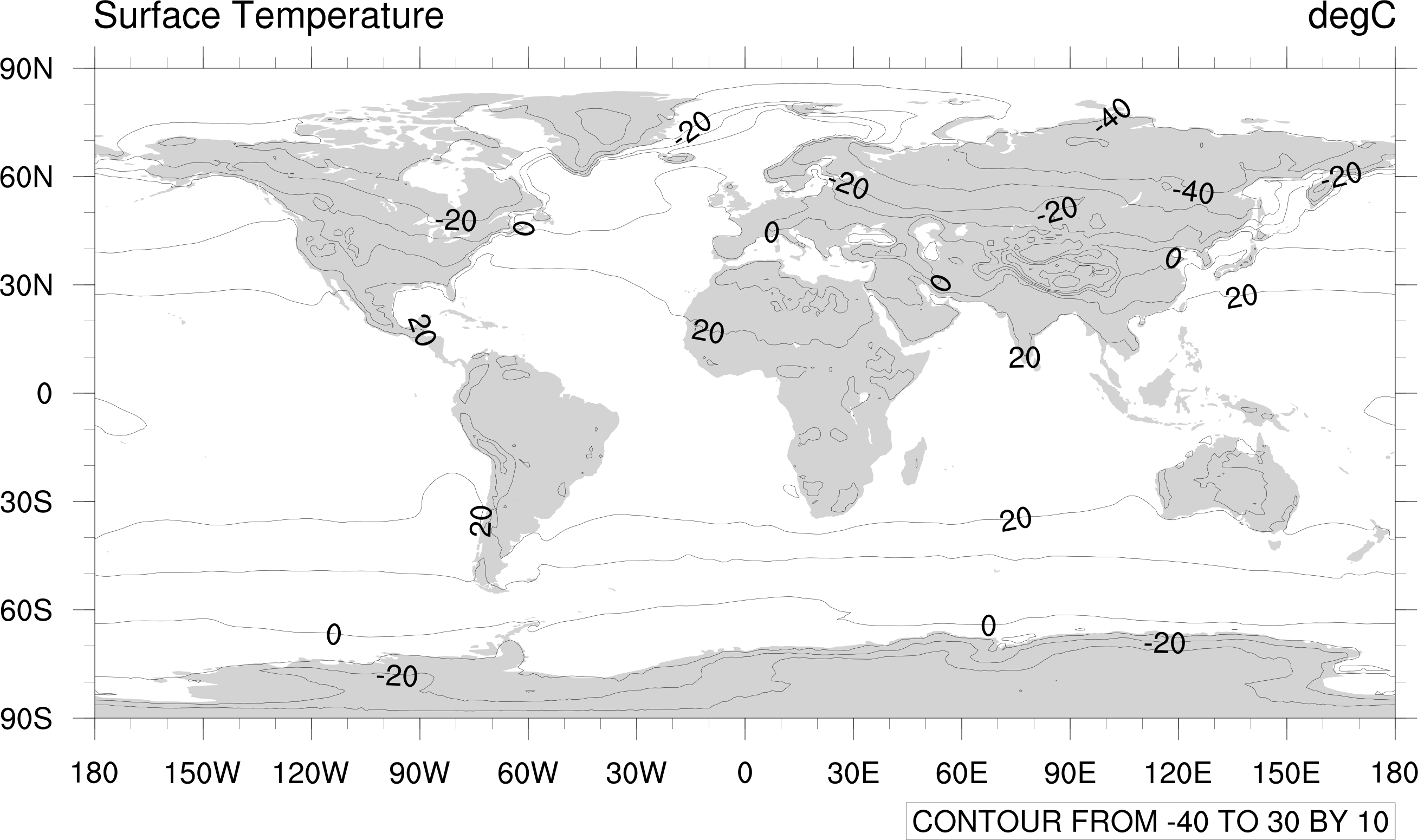
Figure 1 - Click to see a larger image.
Sample NCL script
;----------------------------------------------------------------------
; This script creates a simple line contour plot of the first timestep
; of the "ts" variable on the given NetCDF file.
;----------------------------------------------------------------------

load "$NCARG_ROOT/lib/ncarg/nclscripts/csm/gsn_code.ncl"
load "$NCARG_ROOT/lib/ncarg/nclscripts/csm/gsn_csm.ncl"

begin
;---Open file and read data
  dir      = "/glade/u/sampledata/ncl/CESM/CAM5/"
  filename = "ts_Amon_CESM1-CAM5_historical_r1i1p1_185001-200512.nc"
  a        = addfile(dir+filename,"r")

  ts       = a->ts(0,:,:)            ; Read first time step
  ts       = ts-273.15               ; convert from Kelvin->Celsius
  ts@units = "degC"

;---Look at the variable's metadata, if desired
  printVarSummary(ts)

;---Open file or window to send graphical output to.
  wks = gsn_open_wks("png","contour_ts_line")   ; "png", "ps", "pdf", "x11"

;---Create a default line contour plot.
  res  = True
  plot = gsn_csm_contour_map(wks,ts,res)

end
Example 2
Using a different script, you can create a more interesting visualization with the data that was used in the first example.
Make an NCL script file named contour_ts_color.ncl using the sample script below.
When you run it on Casper, the output to your working directory will be a color-filled contour (Figure 2) called contour_ts_color.png.
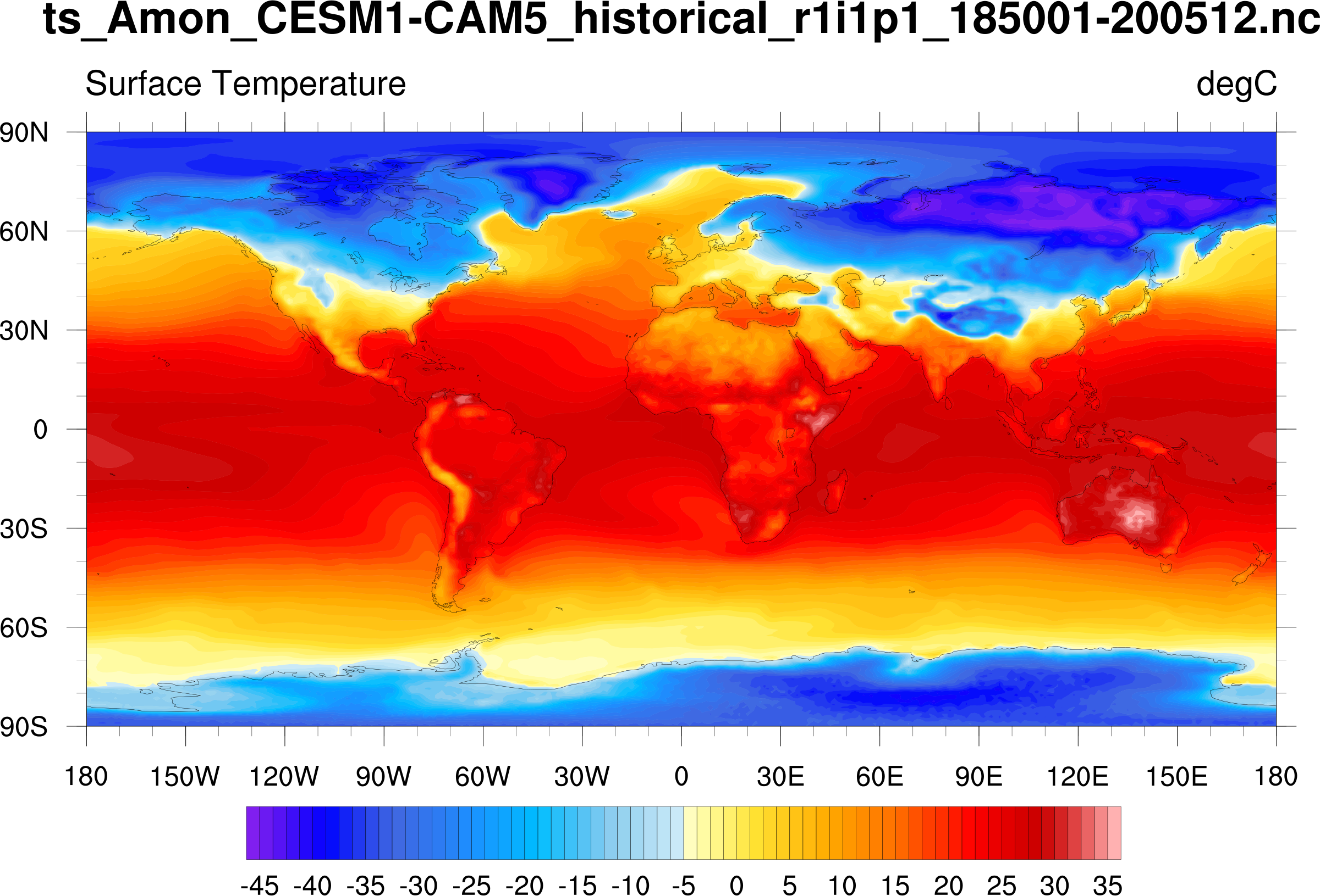
Figure 2 - Click to see a larger image.
Sample NCL script
;----------------------------------------------------------------------
; This script creates filled contour plot of the first timestep of
; the "ts" variable on the given NetCDF file.
;----------------------------------------------------------------------

load "$NCARG_ROOT/lib/ncarg/nclscripts/csm/gsn_code.ncl"
load "$NCARG_ROOT/lib/ncarg/nclscripts/csm/gsn_csm.ncl"

begin
;---Open file and read data
  dir      = "/glade/u/sampledata/ncl/CESM/CAM5/"
  filename = "ts_Amon_CESM1-CAM5_historical_r1i1p1_185001-200512.nc"
  a        = addfile(dir+filename,"r")

  ts       = a->ts(0,:,:)        ; Read first time step.
  ts       = ts-273.15           ; Convert from Kelvin -> Celsius.
  ts@units = "degC"

;---Look at the variable's metadata, if desired
  printVarSummary(ts)

;---Open file or window to send graphical output to.
  wks = gsn_open_wks("png","contour_ts_color")   ; "png", "ps", "pdf", "x11"

;---Set some graphical resources to customize the contour plot.
  res                   = True

  res@gsnMaximize       = True        ; Maximize plot in frame

  res@cnFillOn          = True        ; Turn on contour fill
  res@cnLinesOn         = False       ; Turn off contour lines
  res@cnLineLabelsOn    = False       ; Turn off line labels

  res@tiMainString      = filename    ; Add a main title

  res@gsnAddCyclic      = True        ; Add longitude cyclic point

;--Set the contour levels using "nice_mnmxintvl" function.
  mnmxint = nice_mnmxintvl( min(ts), max(ts), 18, False)
  res@cnLevelSelectionMode = "ManualLevels"
  res@cnMinLevelValF       = mnmxint(0)
  res@cnMaxLevelValF       = mnmxint(1)
  res@cnLevelSpacingF      = mnmxint(2)/4.  ; Decrease spacing for more levels

;---Create and draw the plot.
  plot = gsn_csm_contour_map(wks,ts,res)
end